Near-to-Far Field Transformation For Two Dimension FDTD

Using the near-field data obtained in a single FDTD modeling run, this transformation efficiently and accurately calculates the complete far-field bistatic scattering response of an illuminated structure for a single illumination angle, or the complete radiation pattern of an antenna. In other words, these is no need to extend the FDTD lattice to the far field to obtain far-field data.
In fact, the equivalent electric and magnetic currents tangential to any closed contour surrounding a two-dimensional TM electromagnetic wave interaction structure is sufficient to obtain the far field via a simple integration of these currents around the contour. This idea, illustrated in Fig.1, forms the basis of the surface equivalence theorem.

(a) Original interaction geometry (b) equivalent problem
Fig.1 Definition of electromagnetic fields and equivalent electric and magnetic virtual currents for the surface equivalence theorem.

Applied this concept, the program fd2d_004 calculated the RCS for three structures respectively.
Case 1: Metal square with a=2*lamda , lamda=1.e-6m , and dx=dy=lamda/40. The plane wave incident from the left, that is the incident angle is 0 degree.

Case 2: Metal square with a=2*lamda, lamda=1.e-6m, and dx=dy=lamda/40. The plane wave incident from the left, that is the incident angle is 45 degree.

Case 3: Dielectric circle with r=2*lamda, lamda=1.e-6m, epsr=3.5 and dx=dy=lamda/40 . The plane wave incident from the left, the incident angle is 0 degree.

Case 4：Metal-Dielectric composite squares with a1=0.2*lamda, a2=0.4*lamda, lamda=1m, epsr=3.5 and dx=dy=lamda/40.

If you want to get this FDTD program fd2d_004, please contact with me by Email: aifors@126.com

Two Dimensional FDTD Total Scattered Field Formulation

The simulation of plane waves is often of interest in computational electromagnetics. Many problems, such as the calculation of radar cross sections, deal with plane waves. Furthermore, after a distance on the order of tens of wavelengths, the field from most antennas can be approximated as a plane wave.

In order to simulate a plane wave in a 2D FDTD program, the problem space will be divided up into two regions, the total field and the scattered field. There are two primary reasons for doing this: (1) The propagating plane wave should not interact with the absorbing boundary conditions; (2) the load on the absorbing boundary conditions should be minimized. These boundary conditions are not perfect, i.e. a certain portion of the impinging wave is reflected back into the problem space. By subtracting the incident field, the amount of the radiating field hitting the boundary is minimized, thereby reducing the amount of error.

Figure 1 illustrates how this is accomplished.

First note that there is an auxiliary one-dimensional buffer called the incident array. Because this is a one-dimensional array, it is easy to generate a plane wave: a source point is chosen and the incident Ez field is just added at that point. Then a plane wave propagates away in both directions. Since it is a one-dimensional array, the boundary conditions are perfect.

The program fd2d_003 implements these algorithms with an incident plane wave. Fig.2 and Fig.3 illustrates the propagation of a Gaussian pulse through the problem space at 0 and 90 degree respectively.

Fig.2 the plane wave with the incident angle 0 degree

Fig.3 the plane wave with the incident angle 45 degree

If you want to get this FDTD program fd2d_003, please contact with me by Email: aifors@126.com

The Perfectly Matched Layer (PML)

Up to now, we have only briefly mentioned the issue of absorbing boundary conditions (ABCs). Actually, one of the most flexible and efficient ABCs is the perfectly matched layer (PML) developed by Berenger. The basic idea is this: if a wave is propagating in medium A and it impinges upon medium B, the amount of reflection is dictated by the intrinsic impedances of the two media

If these two media have the equal impedances, the reflection coefficient would be zero and no reflection would occur. This still doesn’t solve our problem, because the pulse will continue propagating in the new medium. What we really want is a medium that is also lossy so the pulse will die out before it hits the boundary. This is accomplished by making both permittivity and permeability of Eq. (2) complex, because the imaginary part represents the part that causes decay.
The PML is implemented in the program fd2d_002. Figure 1 illustrates the effectiveness of an 5-layer PML with the source in the center of problem space.

If you want to get this FDTD program fd2d_002, please contact with me by Email: aifors@126.com.

Two-Dimensional FDTD Simulation

Once again, we will start with the normalized Maxwell’s equations, assume that the structure being modeled extends to infinity in the z-direction. If the incident wave is also uniform in the z-direction, then all partial derivatives of the fields with respect to z must equal zero. Under these conditions, the full set of Maxwell’s curl equations for TMz mode.

As in one-dimensional simulation, it is important that there is a systematic interleaving of the fields to be calculated. This is illustrated in Fig.1. Putting Eqs. (1)~(3) into the finite differencing scheme results in the following difference equations.

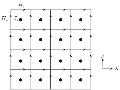
Fig.1 Interleaving of the E and H fields for the two-dimensional TM formulation

The program fd2d_001 implements the above equations. It has a simple Gaussian pulse source that is generated in the middle of the problem space. Fig.2 demonstrates a simulation for the different time steps
!* FD2D_001 2D FDTD simulation in free space *!
Module common_data
implicit none
!Calculate region
integer,save:: Imin,Imax,Jmin,Jmax
!constant
real,parameter:: Eps0=8.854e-12,Mu0=1.25663706e-6
real,parameter:: C0=3.e8,Z0=377.,Pi=3.1415926536d0
!source parameter
real,save ::SourceT0,SourceT
!MAXIMUM NUMBER OF TIME STEPS
integer,parameter:: timestop=250
!grid size,timestep
real,save:: dx,dy,dt
!variables for Field
real,dimension(:,:),allocatable,save:: Ez,Hx,Hy
endmodule common_data

program main
use common_data
implicit none
integer ntime
call pre_processing
!MAIN LOOP FOR FIELD COMPUTATIONS AND DATA SAVING
do Ntime=1,timestop
call Ezfd2d(Ntime)
call Hxfd2d
call Hyfd2d
enddo
call savedata
end

subroutine pre_processing
use common_data
implicit none
Imin=-150;Imax=150
Jmin=-150;Jmax=150
allocate (Ez(Imin:Imax,Jmin:Jmax))
allocate (Hx(Imin:Imax,Jmin:Jmax))
allocate (Hy(Imin:Imax,Jmin:Jmax))
Ez=0.;Hx=0.;Hy=0.
dx=1.e-2;
dy=dx
dt=dx/2./c0
SourceT0=120;SourceT=50
return
end

subroutine Ezfd2d(n)
use common_data
implicit none
integer i,j,n
do i=Imin,Imax-1
do j=Jmin,Jmax-1
Ez(i,j)=Ez(i,j)+(Hy(i+1,j)-Hy(i,j))*dt/dx/Eps0
* -(Hx(i,j+1)-Hx(i,j))*dt/dy/Eps0
enddo
enddo
Ez(0,0)=exp(-((n-1)*1.-SourceT0)**2/SourceT**2)
return
end

subroutine Hxfd2d
use common_data
implicit none
integer i,j
do i=Imin,Imax-1
do j=Jmin+1,Jmax-1
Hx(i,j)=Hx(i,j)-(Ez(i,j)-Ez(i,j-1))*dt/dy/Mu0
enddo
enddo
return
end

subroutine Hyfd2d
use common_data
implicit none
integer i,j
do i=Imin+1,Imax-1
do j=Jmin,Jmax-1
Hy(i,j)=Hy(i,j)+(Ez(i,j)-Ez(i-1,j))*dt/dx/Mu0
enddo
enddo
return
end

subroutine savedata
use common_data
implicit none
integer j
open(1,file='ez.m')
open(2,file='xgrid')
open(3,file='ygrid')
write(1,*) 'z=['
do j=Jmin,Jmax-1
write(1,100) Ez(Imin:Imax-1,j)
enddo
write(1,*) ']'
write(2,*) (j,j=Imin,Imax-1)
write(3,*) (j,j=Jmin,Jmax-1)
close(1)
close(2)
close(3)
100 format(99999(1x,E12.4))
return
end

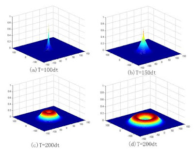
Fig.2 Results of a simulation using the program fd2d_001.

Total-Field/Scattered-Field Formulation in One-Dimension FDTD

The total-field/scattered-field (TF/SF) formulation resulted from attempts to realize a plane-wave source that avoid the difficulties caused by using either hard sources or the initial-condition approach. The TF/SF formulation is based on the linearity of Maxwell’s equations.

We note that the finite-difference operations of the Yee algorithm can be applied with equal validity to the incident field, the scattered field, and the total field. This property permits zoning the Yee space lattice into two distinct regions (as shown in Fig.1): Region 1, where total fields are assumed to be stored in the computer memory; and Region 2 (surrounding Region 1), where scattered fields are assumed stored in the computer memory. Regions 1 and 2 are separated by a nonphysical virtual surface that serves to connect the fields in each region, called the total/scattered field boundary.

Fig.1 Total/Scattered field zoning in one-dimensional x-directed FDTD space lattice.

Based on these formulations, the total-field/scattered-field boundary condition has been implemented at both side of the array in the program FD1D_003, list as follow:
!* FD1D_003 1D FDTD simulation in free space *!
!* Absorbing Boundary Condition added *!
!* Total Scattered Boundary Condition added *!
Module common_data
implicit none
!Calculate region
integer,save:: Imin,Imax,Itmin,Itmax
!constant
real,parameter:: Eps0=8.854e-12,Mu0=1.25663706e-6
real,parameter:: C0=3.e8,Z0=377.,Pi=3.1415926536d0
!source parameter
real,save ::SourceT0,SourceT
!MAXIMUM NUMBER OF TIME STEPS
integer,parameter:: timestop=300
!grid size,timestep
real,save:: dx,dt
!variables for Field
real,dimension(:),allocatable,save:: Ez,Hy
!Variables for absorbing boundary
real,dimension(:),allocatable,save:: ABC
endmodule common_data

program main
use common_data
implicit none
integer ntime,i
call pre_processing
!MAIN LOOP FOR FIELD COMPUTATIONS AND DATA SAVING
DO Ntime=1,timestop
call Ezfd1d
call EzTSBC(Ntime)
call EzABC
call Hyfd1d
call HyTSBC(Ntime)
enddo
call savedata
end

subroutine pre_processing
use common_data
implicit none
Imin=-300;Imax=300
Itmin=-200;Itmax=200
allocate(Ez(Imin:Imax))
allocate(Hy(Imin:Imax))
allocate(ABC(1:4))
Ez=0.;Hy=0.;ABC=0.
dx=1.e-2;
dt=dx/2./c0
SourceT0=120;SourceT=50
return
end

subroutine Ezfd1d
use common_data
implicit none
integer i,n
do i=Imin+1,Imax-1
Ez(i)=Ez(i)+(Hy(i-1)-Hy(i))*dt/dx/Eps0
enddo
return
end

subroutine EzTSBC(n)
use common_data
implicit none
integer n,rn
Ez(Itmin)=Ez(Itmin)+exp(-((n-1)*1.-SourceT0)**2/SourceT**2)
* *dt/dx/Eps0/z0
rn=n-802
if(rn.gt.0) then
Ez(Itmax)=Ez(Itmax)-exp(-((rn-1)*1.-SourceT0)**2/SourceT**2)
* *dt/dx/Eps0/z0
endif
return
end

subroutine EzABC
use common_data
implicit none
Ez(Imin)=ABC(2)
ABC(2)=ABC(1)
ABC(1)=Ez(Imin+1)
Ez(Imax)=ABC(4)
ABC(4)=ABC(3)
ABC(3)=Ez(Imax-1)
return
end

subroutine Hyfd1d
use common_data
implicit none
integer i
do i=Imin,Imax-1
Hy(i)=Hy(i)-(Ez(i+1)-Ez(i))*dt/dx/Mu0
enddo
return
end

subroutine HyTSBC(n)
use common_data
implicit none
integer n,rn
Hy(Itmin-1)=Hy(Itmin-1)+exp(-((n-1)*1.-SourceT0)**2/SourceT**2)
* *dt/dx/Mu0
rn=n-801
if(rn.gt.0) then
Hy(Itmax)=Hy(Itmax)-exp(-((rn-1)*1.-SourceT0)**2/SourceT**2)
* *dt/dx/Mu0
endif
return
end

subroutine savedata
use common_data
implicit none
integer i
open(1,file='ex')
open(2,file='z_cell')
write(1,*) (Ez(i),i=Imin,Imax)
write(2,*) (i,i=Imin,Imax)
close(1)
close(2)
return
end

Fig.2 Action of total-field/scattered-field zoning for a one-dimensional linear Yee grid.